PRODUCTION 

JOIN BEST SSC EXAMS COACHING CENTERS IN VIJAYAWADA, BEST SSC CGL TRINING CENTERS IN VIJAYAWADA

Production: Combining inputs in order to get the output is production. 
Production Function: It is the functional relationship between inputs and output in a given state of technology. Q= f(L,K) 
Q is the output, L: Labor, K: Capital 
Fixed Factor: The factor whose quantity remains fixed with the level of output. 
Variable Factor: Those inputs which change with the level of output. 

PRODUCTION FUNCTION AND TIME PERIOD 

1. Production function is a long period production function if all the inputs are varied. 
2. Production function is a short period production function if few variable factors are combined with few fixed factors. 
 

JOIN BEST SSC CGL EXAMS COACHING CENTER IN VIJAYAWADA,

Concepts of product: 
Total Product- Total quantity of goods produced by a firm / industry during a given period of time with given number of inputs. 
Average product = output per unit of variable input. 
APP = TPP / units of variable factor 
Average product is also known as average physical product. 
Marginal product (MP): refers to addition to the total product, when one more unit of variable factor is employed. 
MPn = TPn – TPn-1 
MPn = Marginal product of nth unit of variable factor 
TPn = Total product of n units of variable factor 
TPn-1= Total product of (n-1) unit of variable factor. 
n=no. of units of variable factor 
MP = ΔTP / Δn 
We derive TP by summing up MP TP = ΣMP 

SHORT RUN PRODUCTION FUNCTION LAW OF VARIABLE PROPORTION OR RETURNS TO A VARIABLE FACTOR 

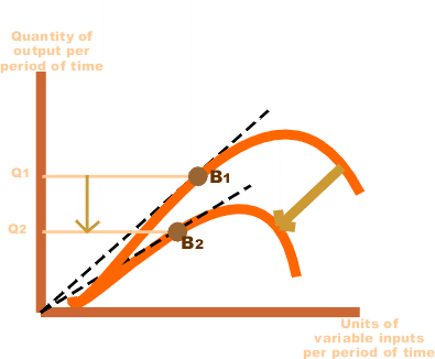
Statement of law of variable proportion: In short period, when only one variable factor is increased, keeping other factors constant, the total product (TP) initially increases at an increasing rate, then increases at a decreasing rate and finally TP decreases. 
MPP initially increase then falls but remains positive then 3rd phase becomes negative. 

Phase I / Stage I / Increasing returns to a factor.                                                      
• TPP increases at an increasing rate 
• MPP also increases. 

Phase II / Stage II / Diminishing returns to a factor 
• TPP increases at decreasing rate 
• MPP decreases / falls 
• This phase ends when MPP is zero & TPP is maximum 

Phase III / Stage III / Negative returns to a factor 
• TPP diminishes / decreases 
• MPP becomes negative. 

Reasons for increasing returns to a factor 
• Better utilization of fixed factor 
• Increase in efficiency of variable factor. 
• Optimum combination of factors 

Reasons for diminishing returns to a factor 
• Indivisibility of factors. 
• Imperfect substitutes. 

Reasons for negative returns to a factor 
• Limitation of fixed factors 
• Poor coordination between variable and fixed factor 
• Decrease in efficiency of variable factors

Relation between MPP and TPP                                                                              
• As long as MPP increases, TPP increases at an increasing rate. 
• When MPP decreases, TPP increases diminishing rate. 
• When MPP is Zero, TPP is maximum. 
• When MPP is negative, TPP starts decreasing. 

Long-run production function - Returns to Scale 
In the long run, all factors can be changed. Returns to scale studiesthe changes in output when all factors or inputs are changed. An increase in scale means that all inputs or factors are increased in the sameproportion. 

Three phases of returns to scale 
The changes in output as a result of changes in the scale can be studied in 3 phases. They are 
(i) Increasing returns to scale(ii) Constant returns to scale (iii) Decreasing returns to scale 

BEST SSC CHSL TRINING CENTER IN VIJAYAWADA

Increasing returns to scale 
If the increase in all factors leads to a more than proportionate increase in output, it is called increasing returns to scale. For example, 
if all the inputs are increased by 5%, the output increases by more than 5% i.e. by 10%. In this case the marginal product will be rising. 

Constant returns to scale 
If we increase all the factors (i.e. scale) in a given proportion, the output will increase in the same proportion i.e. a 5% increase in all the factors will result in an equal proportion of 5% increase in the output. Here the marginal product is constant. 

BEST SSC CHSL EXAMS TRINING CENTERS IN VIJAYAWADA
 

Decreasing returns to scale 
If the increase in all factors leads to a less than proportionate increase in output, it is called decreasing returns to scale i.e. if all the factors are increased by 5%, the output will increase by less than 5% i.e. by 3%. In this phase marginal product will be decreasing. 
The Cobb – Douglas Production Function 
The simplest and the most widely used production function in economics is the Cobb-Douglas production function. It is a statistical production function given by professors C.W. Cobb and P.H. Douglas. 
The Cobb-Douglas production function can be stated as follows 
Q = bLaC1− ain which 
Q = Actual output L = LabourC = Capitalb = number of units of Laboura = Exponentof labour1-a = Exponentof Capital 
According to the above production function, if both factors of production (labour and capital) are increased by one percent, the output 
(total product) will increase by the sum of the exponents of labour and capital i.e. by (a+1-a). Since a+1-a =1, according to the equation, when the inputs are increased by one percent, the output also increases by one percent. Thus the Cobb Douglas production function explains only constant returns to scale. 
In the above production function, the sum of the exponents shows the degree of “returns to scale” in production function. 
a + b >1 : Increasing returns to scale 
a + b =1 : Constant returns to scale 
a + b <1 : Decreasing returns to scale 

 BEST SSC CHSL EXAMS TRINING CENTERS IN VIJAYAWADA

COST 

Cost of production : Expenditure incurred on various inputs to produce goods and services. 

Cost function : Functional relationship between cost and output. 
C=f(q) Where f=functional relationshipwherec= cost of production q=quantity of product 

Money cost : Money expenses incurred by a firm for producing a commodity or service. 

Explicit cost : Actual payment made on hired factors of production. For example wages paid to the hired labourers, rent paid for hired accommodation, cost of raw material etc. 

Implicit cost : Cost incurred on the self - owned factors of production. For example, interest on owners capital, rent of own building, salary for the services of entrepreneur etc. 

Opportunity cost : is the cost of next best alternative foregone / sacrificed. 

BEST SSC CHSL EXAMS CENTERS
 

Fixed cost : are the cost which are incurred on the fixed factors of production.These costs remain fixed whatever may be the scale of output. These costs are present even when the output is zero. These costs are present in short run but disappear in the long run. 
Total Variable Cost : TVC or variable cost – are those costs which vary directly with the variation in the output. These costs are incurred on the variable factors of production.These costs are also called “prime costs”, “Direct cost” or “avoidable cost”. These costs are zero when output is zero. 

Total cost : is the total expenditure incurred on the factors and non-factor inputs in the production of goods and services.
It is obtained by summing TFC and TVC at various levels of output. 
Relation between TC, TFC and TVC 
1. TFC is horizontal to x axis. 
2. TC and TVC are S shaped (they rise initially at a decreasing rate, then at a constant rate & finally at an increasing rate) due to law of variable proportions. 
3. At zero level of output TC is equal to TFC. 
4. TC and TVC curves parallel to each other. 
Average variable costis the cost per unit of the variable cost of production. AVC = TVC / output. 
AVC falls with every increase in output initially. 
Once the optimum level of output is reached AVC starts rising. 
Average total cost (ATC) or Average cost (AC): refers to the per unit total cost of production. 
Marginal cost:refers to the addition made to total cost when an additional unit of output is produced. 
MCn = TCn-TCn-1 or MC = ΔTC / ΔQ Note : MC is not affected by TFC. 
Relationship between AC and MC 
• Both AC & MC are derived from TC 
• Both AC & MC are “U” shaped (Law of variable proportion) 
• When AC is falling MC also falls & lies below AC curve. 
• When AC is rising MC also rises & lies above AC 
• MC cuts AC at its minimum where MC = AC 

BEST SSC CGL EXAMS CENTERS

Revenue 

Revenue:- Money received by a firm from the sale of a given output in the market. 
Total Revenue: Total sale receipts or receipts from the sale of given output. 
TR = Quantity sold × Price (or) output sold × price 
Average Revenue: Revenue or Receipt received per unit of output sold. 
?    AR = TR / Output sold 
?    AR and price are the same. 
?    TR = Quantity sold × price or output sold × price 
?    AR = (output / quantity × price) / Output/ quantity 
?    AR= price 
?    AR and demand curve are the same. Shows the various quantities demanded at various prices. 

Marginal Revenue: Additional revenue earned by the seller by selling an additional unit of output. 
• MRn = TR n - TR n-1 • TR = Σ MR 
Relationship between AR and MR(when price remains constant or perfect competition) 
Under perfect competition, the sellers are price takers. Single price prevails in the market. Since all the goods are homogeneous and are sold at the same price AR = MR. As a result AR and MR curve will be horizontal straight line parallel to OX axis. (When price is constant or perfect competition) 
Relation between TR and MR (When price remains constant or in perfect competition) 
When there exists single price, the seller can sell any quantity at that price, the total revenue increases at a constant rate (MR is horizontal to X axis) 
Relationships between AR and MR under monopoly and monopolistic competition(Price changes or under imperfect competition) 
• AR and MR curves will be downward sloping in both the market forms. 
• AR lies above MR. 
• AR can never be negative. 
• AR curve is less elastic in monopoly market form because of no substitutes. 
• AR curve is more elastic in monopolistic market because of the presence of substitutes. 
Relationship between TR and MR. (When price falls with the increase in sale of output) 
• Under imperfect market AR will be downward sloping – which shows that more units can be sold only at a less price. 
• MR falls with every fall in AR / price and lies below AR curve. 
• TR increases as long as MR is positive. 
• TR falls when MR is negative. 
• TR will be maximum when MR is zero 

Break-even point: It is that point where TR = TC or AR=AC. Firm will be earning normal profit. 
Shut down point : A situation when a firm is able to cover only variable costs or TR = TVC 
Formulae at a glance: 
• TR = price or AR × Output sold or TR = Σ MR 
• AR (price) = TR ÷ units sold 
• MR n = MR n – MR n-1 

BEST SSC CHSL EXAMS CENTERS, TOP SSC COACHING CENTERS, ONLINE SSC COACHING, STAFFSELECTION COACHING CENTERS IN VIJAYAWADA.